A Few Common Statistical Distributions

If you are a developer, you might think of statistical distributions as design patterns for statistical analysis. For instance, a normal distribution can concisely, with only two parameters, model a vast variety of phenomena. You won't get a perfect model, but, as George Pox put it:

All models are wrong, some are useful.

Statistical distributions can be seen as an attempt to create simple models that are reusable for many different cases. I think simplicity deserves some emphasis here. In fact, the above quote about all models being wrong is a nice one, but, in a paper by George Pox there's a sentence I like even more:

Just as the ability to devise simple but evocative models is the signature of the great scientist so overelaboration and overparameterization is often the mark of mediocrity.

Over time, a bunch of reusable models have been created. Let's have a look at the Bernoulli, Binomial, Geometric, Poisson, Exponential, Normal and Log-normal distribution. There are many more, but hey, we have to start somewhere.

The Bernoulli Distribution

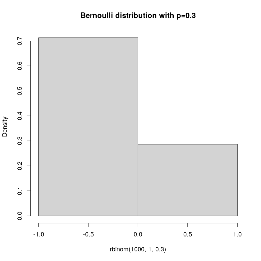
If you think about what a coin toss is, it is an event (coin is thrown up in the air) with two outcomes (heads or tails), and these have equal probability. A Bernoulli distribution can describe probabilities related to a process with such a setup. However, it can do more than that, indeed, it can also handle unequal probabilities for the outcomes. You may think that flipping coins isn't the most important thing to model. But, imagine if your coin flip is rather whether a customer purchases something or not. Also here we have an event (customer visits your shop/website) and two outcomes (purchase/no purchase). These events are unlikely to have equal probability of course, and indeed, your work as a designer is to push up the probability of the desired outcome.

Finally, let us look at the probability mass function (PMF):

\[ \begin{alignat}{1} &X{\sim}\text{Bern}(p)\\ &P(X=x) = p^x(1-p)^{1-x}I_{\{0,1\}}(x) \end{alignat} \]

This function describes the probability associated with the outcomes, which are represented as x=0 or x=1.

The Binomial Distribution

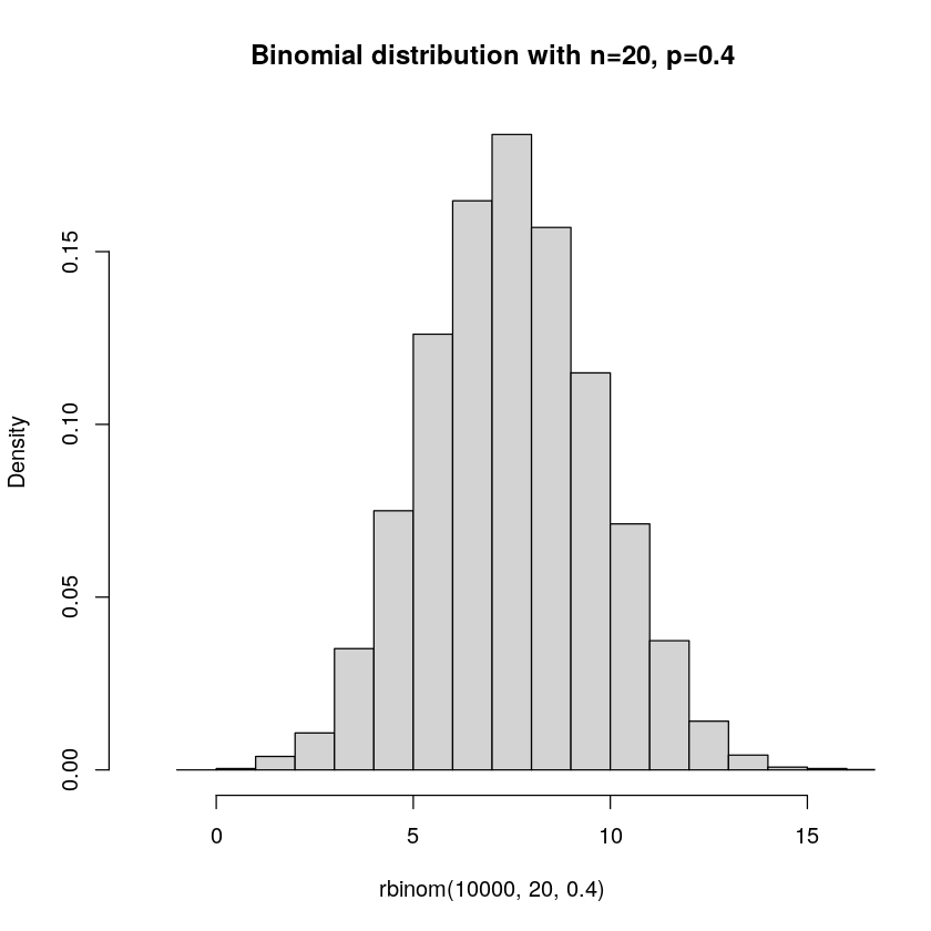
What if we do a bunch of Bernoulli trials? Let us imagine that we toss our coin 10 times. A natural thing to be interested in then is how many coin tosses result in heads or tails. Or, for a website, we might want to ask ourselves: out of all unique sessions, how many resulted in a purchase?

The Binomial distribution is the sum of independent Bernoulli trials. E.g. we toss the coin 10 times. We decide on what success is, and label it 1. E.g. if heads is considered success, the outcome of our series of tosses is the number of heads. In this case, a Binomial distribution allows us to calculate probabilities for how many heads we will get.

Finally, let us look at the probability mass function (PMF):

\[ \begin{alignat}{1} &X{\sim}\text{Bin}(n,p)\\ &P(X=x) = {n\choose x}p^x(1-p)^{n-x}I_{\{0,1,...,n\}}(x) \end{alignat} \]

It is a quite neat function. \(p^x\) is the probability of the successes. \((1-p)^{n-x}\) is the probability of failures. \(n\choose x\) comes from that success can happen at any of the n trials.

The Geometric Distribution

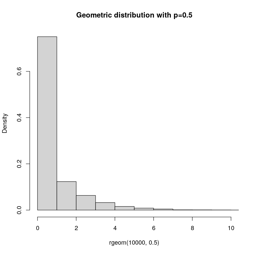
Counting the number of successes given a fixed number of attempts may be interesting for some. But what if we are interested in the number of attempts until our first success? Well, the Geometric distribution is all about that. It gives us the probability of having to do a certain number of attempts until we get our first success. E.g. how many times do we need to toss our coin until we get heads?

Finally, let us look at the probability mass function (PMF):

\[ \begin{alignat}{1} &X{\sim}\text{Geom}(p)\\ &P(X=x) = p(1-p)^{x-1}I_{\{1,2,...\}}(x) \end{alignat} \]

This function nicely represents one success and \(x-1\) failures. No need to count the number of combinations as for the Binomial distribution, since we stop the experiment on the first success, so the success will always come after zero or more failures.

The Poisson Distribution

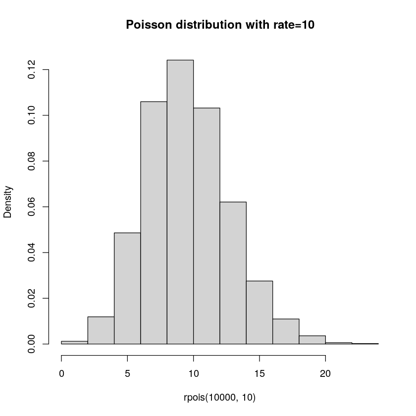
The Bernoulli, Binomial and Geometric distributions are related, all are reasoning about some event with two outcomes. Poisson is instead about the number of events. It is parameterized by the rate of an event, e.g. "5 events per hour". It can then give us the probability of a certain number of events in a time period. E.g. what is the probability of getting 10 events in an hour?

Finally, let us look at the probability mass function (PMF):

\[ \begin{alignat}{1} &X{\sim}\text{Poisson}(rate=\lambda)\\ &P(X=x) = \dfrac{e^{-\lambda}\lambda^x}{x!}I_{\{0,1,...\}}(x) \end{alignat} \]

The Exponential Distribution

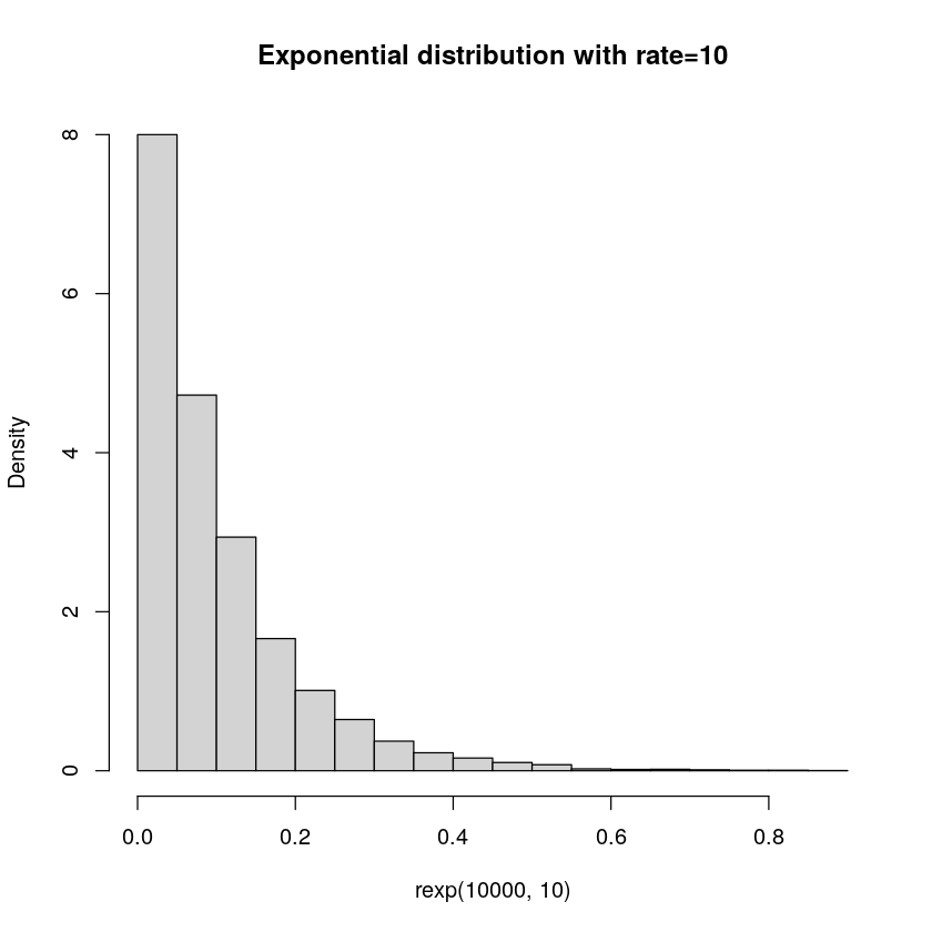
The Poisson distribution describes the number of events in some time period. Exponential can be seen as its best friend, which looks at the time between events. These are naturally related, e.g. if a Poisson distribution has rate parameter 2 per hour, then, naturally, we can expect that it should on average be 30 minutes between events. This time between events is what the Exponential distribution models. And, beautifully enough, you can use the same parameter as for the Poisson distribution.

Finally, let us look at the probability density function (PDF):

\[ \begin{alignat}{1} &f(x) = \lambda e^{-\lambda x}I_{\{0,\infty\}}(x) \end{alignat} \]

Note that we are now dealing with a PDF rather than PMF, since the exponential distribution is an example of a continuous distribution, in contrast to the discrete presented before.

The Normal Distribution

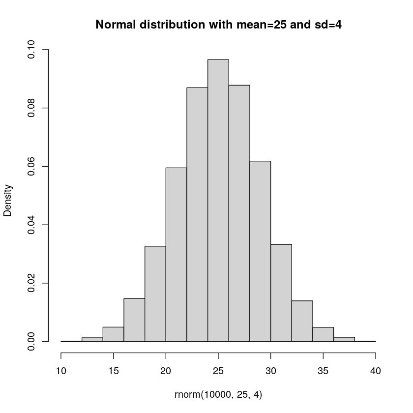
Sometimes known as the bell-curve, the normal distribution is famous to be seen everywhere. Whenever you think about that something can be +- a bit, you are likely thinking of something with a normal distribution. An example would be the height of penguins. It is not unreasonable to suspect that there will be some most common height, and then penguins will be shorter and taller, but much shorter or much taller, is increasingly rare.

Finally, let us look at the probability density function (PDF):

\[ \begin{alignat}{1} &f(x) = \frac{1}{\sqrt{2\pi\sigma^2}}e^{-\frac{1}{2\sigma^2}(x-\mu)^2} \end{alignat} \]

The Log-Normal Distribution

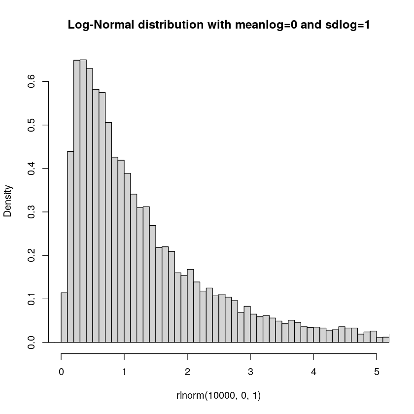
There's a little bug with the normal distribution. What if something is very skewed? Perhaps the length of a text message? It isn't unreasonable to expect that there might be a bias towards shorter messages. And the length of messages can naturally not be negative. While it could be equally likely that messages are a bit shorter and longer, it could also very well be that short messages are more common and longer are increasingly less likely. Well, a log-normal distribution can help us model this!

Finally, let us look at the probability density function (PDF):

\[ \begin{alignat}{1} &f(x) = \frac{1}{x\sigma\sqrt{2\pi}}e^{-\frac{(\ln{x}-\mu)^2}{2\sigma^2}} \end{alignat} \]

Noteworthy is that the log-normal distribution and normal distribution have a mapping between each other:

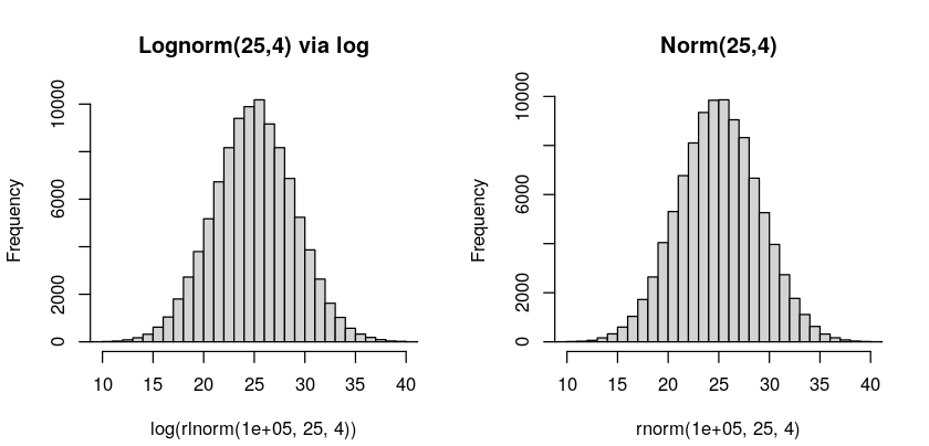
This means that you can transform between these, for instance to perform analyses on the normal distribution rather than log-normal, if you find that more convenient. You simply take the log of your data from a log-normal distribution to get a normal distribution. Or, take \(e^x\) where x is your data from a normal distribution, which you wish to represent as a log-normal distribution.

Conclusion

I hope you enjoyed learning about the Bernoulli, Binomial, Geometric, Poisson, Exponential, Normal and Log-Normal distribution. That is quite a few, and there are many more. It is quite overwhelming, but as with anything, if you are interested and spend time with these, they will feel like tools in your toolbox rather than a burden to remember and understand.